Algebra
1. Defining Sets
One of the most fundamental concepts in Algebra is the concept of a set. This video introduces the concept of a set and various methods for defining sets.

2. Set Equality and Subsets
Sets can be related to each other in different ways. This chapter describes the set relations of equality, subset, superset, proper subset, and proper superset.

3. Venn Diagrams, Unions, and Intersections
Venn diagrams are an important tool allowing relations between sets to be visualized graphically. This chapter introduces the use of Venn diagrams to visualize intersections and unions of sets, as well as subsets and supersets.

4. Complement and Relative Complement
The complement of a set is the collection of all elements which are not members of that set. Although this operation appears to be straightforward, the way we define 'all elements' can significantly change the results.

5. Symmetric Difference
The symmetric difference of two sets is the collection of elements which are members of either set but not both - in other words, the union of the sets excluding their intersection.

6. Interval Notation and the Number Line
Although Venn diagrams are a useful way to visualize sets whose elements can be any type of object, interval notation and the number line are best suited for describing sets of real numbers used in Algebra.

7. Bounded versus Unbounded Intervals
Bounded intervals may be either open or closed. Closed intervals contain a maximum and minimum number, but why is it impossible to find the maximum or minimum number in an open interval?

8. Unions of Intervals
Interval notation is often the simplest way to describe sets of real numbers as regions on the number line. Some sets which cannot be represented by a single interval can be written in interval notation as the union of two or more intervals.

9. Cartesian Products, Ordered Pairs and Triples
Cartesian products can create sets of ordered pairs which correspond to points in 2-dimensional space, or ordered triples which correspond to points in 3-dimensional space. These sets form the logical foundation of the Cartesian coordinate system.

10. The Cartesian Coordinate System
The Cartesian coordinate system, formed from the Cartesian product of the real number line with itself, allows algebraic equations to be visualized as geometric shapes in two or three dimensions.

11. Cartesian Coordinates in Three Dimensions
Just as the Cartesian plane allows sets of ordered pairs to be graphically displayed as 2-dimensional objects, Cartesian space allows us to visualize sets of ordered triples in three dimensions.

12. Binary Relations
Fundamental to Algebra is the concept of a binary relation. This concept is closely related to the concept of a function.

13. Domain and Range of Binary Relations
Two sets which are of primary interest when studying binary relations are the domain and range of the relation.

14. Scatter Plots
Scatter plots are a powerful method of visualizing relations between sets of numeric values. As an example, trends in a binary relation between the height and weight of a group of people could be graphed and analyzed by using a scatter plot.

15. Functions
Functions can be thought of as mathematical machines, which when given an element from a set of permissible inputs, always produce the same element from a set of possible outputs.

16. Real-Valued Functions of a Real Variable
Although the domain and codomain of functions can consist of any type of objects, the most common functions encountered in Algebra are real-valued functions of a real variable, whose domain and codomain are the set of real numbers, R.

17. Vertical Line Test
A graph in Cartesian coordinates may represent a function or may only represent a binary relation. The 'vertical line test' is a simple way to determine whether or not a graph represents a function.

18. Multivariable Functions
Although many familiar functions process a single input variable to produce a single output value, multivariable functions can be created whose output depends upon multiple input variables.

19. Linear Equations: y = mx
Equations of the form y = mx describe lines in the Cartesian plane which pass through the origin. The fact that many functions are linear when viewed on a small scale, is important in branches of mathematics such as calculus.

20. Slope-Intercept Form
Linear equations of the form y = mx+b can describe any non-vertical line in the Cartesian plane. The constant m determines the line's slope, and the constant b determines the y intercept and thus the line's vertical position.

21. Slope
Slope is a fundamental concept in mathematics. Slope if often defined as 'the rise over the run' ... but why?

22. Point-Slope Form
The point-slope form of the equation for a line can describe any non-vertical line in the Cartesian plane, given the slope and the coordinates of a single point which lies on the line.

23. Two-Point Form
The two-point form of the equation for a line can describe any non-vertical line in the Cartesian plane, given the coordinates of two points which lie on the line.

24. Standard Form
The standard form of the equation for a line Ax + By = C can describe any line in the Cartesian plane, including vertical lines. The constants A, B and C have no special meaning, but in combination they tell us many things about the line's graph.

25. Linear Equations in the Real World
Linear equations can be used to solve many types of real-world problems. In this episode, the water depth of a pool is shown to be a linear function of time and an equation is developed to model its behavior.

26. Solving Literal Equations
Literal equations are formulas for calculating the value of one unknown quantity from one or more known quantities.

27. Solving Problems with Linear Equations
How do we create linear equations to solve real-world problems? This video explains the process.

28. Solving Motion Problems with Linear Equations
Based upon the definition of speed, linear equations can be created which allow us to solve problems involving time, distance, and constant speeds.

29. Understanding Percentages
Percentages are one method of describing a fraction of a quantity. The percent is the numerator of a fraction whose denominator is understood to be one-hundred.

30. Solving Percentage Problems with Linear Equations
Many real-world problems involve percentages. This lecture shows how Algebra is used to solve problems involving percent change and profit-and-loss.

31. Calculating Mixtures of Solutions
This lecture shows how Algebra is used to solve problems involving mixtures of solutions of different concentrations.

32. Solving Mixture Problems with Linear Equations
Mixture problems can involve mixtures of things other than liquids. This video shows how Algebra is used to solve problems involving various types of mixtures.

33. Parallel Lines
Parallel lines have the same slope and no points in common. However, it is not always obvious whether two equations describe parallel lines or the same line.

34. Perpendicular Lines
Perpendicular lines have slopes which are negative reciprocals of each other, but why?

35. Systems of Linear Equations in Two Variables
The points of intersection of two graphs represent common solutions to both equations. Finding these intersection points is an important tool in analyzing physical and mathematical systems.

36. Solving Systems of Equations by Substitution
A system of two equations in x and y can be solved by rearranging one equation to represent x in terms of y, and then substituting this expression for x into the other equation to create an equation with only the variable y. This equation can then be solved to find y's value which can then be substituted back into either equation to find the value of x.

37. Solving Systems of Equations by Elimination
Systems of two equations in x and y can be solved by adding the equations to create a new equation with one variable eliminated. That equation can then be solved to find the value of that variable.

38. Why the Elimination Method Works
This chapter takes a geometric look at the logic behind adding equations, the essential technique used when solving systems of equations by elimination.

39. Inconsistent, Dependent, & Independent Systems
Systems of two linear equations in two variables can have a single solution, no solutions, or an infinite number of solutions. This chapter explains why.

40. Solving Inconsistent or Dependent Systems
When solving a system of linear equations in x and y with a single solution, we get a unique pair of values for x and y. But what happens when we try to solve a system with no solutions or an infinite number of solutions?

41. Using Systems of Equations Versus One Equation
When should a system of equations with multiple variables be used to solve an Algebra problem, instead of using a single equation with a single variable?

42. Visualizing Linear Equations in Three Variables
Just as the graph of a linear equation in two variables is a line in the Cartesian plane, the graph of a linear equation in three variables is a plane in Cartesian space.

43. Types of Linear Systems in Three Variables
This video illustrates eight ways in which planes in the graph of a system of three linear equations in three variables can be oriented, thus creating different types of solution sets.

44. Solving Systems of Equations in Three Variables
Systems of three linear equations in three variables can be solved using the same techniques of substitution and elimination used to solve systems of two linear equations in two variables.

45. Three Variable Systems with Infinite or Null Solution Sets
When solving a system of linear equations with a single solution, we get a unique value for each variable. But how do we recognize when a system of equations has infinitely many solutions or no solutions?

46. Parametric Equations
In order to mathematically describe a line in 3-dimensional space, we need a way to define the values of the three coordinates at every point along the line. This can be done by creating a group of 'parametric equations'.

47. Describing Infinite Solution Sets Parametrically
When the graph of the solutions of a system of linear equations in three variables is a line in Cartesian space, the solutions can be described either by a group of three parametric equations, or a parametric ordered-triple. This lecture describes the process of calculating that parametric representation.

48. A Geometrical View of the Elimination Method
When the elimination method is used to solve a system of linear equations, viewing the geometrical changes that happen to the system during this process can give insight into the mechanisms which underlie the logic behind the algebraic method of elimination of variables.

49. Three Variable Systems in the Real World - Problem 1
Algebra 49, 50 and 51 present three real-world problems which can be solved using systems of three linear equations in three variables. This chapter shows how prices of three individual items can be determined, given three combinations of quantities of each item and each combination's total cost.

50. Three Variable Systems in the Real World - Problem 2
Algebra 49, 50 and 51 present three real-world problems which can be solved using systems of three linear equations in three variables. This chapter shows how the parameters of an equation for a parabola can be determined, given three points which satisfy the equation.

51. Three Variable Systems in the Real World - Problem 3
Algebra 49, 50 and 51 present three real-world problems which can be solved using systems of three linear equations in three variables. This chapter shows how the parameters of an equation for a circle can be determined, given three points which satisfy the equation.

52. An Introduction to Matrices
Matrices are an important class of mathematical object used in many branches of mathematics, science and engineering. This lecture also introduces augmented matrices, a compact easy-to-manipulate representation of systems of linear equations, and a valuable tool for solving these systems.

53. Elementary Row Operations
Once a system of linear equations has been converted to augmented matrix form, that matrix can then be transformed using elementary row operations into a matrix which represents a simpler system of equations with the same solutions as the original system. This lecture introduces the three elementary row operations used to achieve this transformation.

54. Gaussian Elimination
A system of linear equations represented as an augmented matrix can be simplified through the process of Gaussian elimination to row echelon form. At that point the matrix can be converted back into equations which are simpler and easy to solve through back substitution.

55. Gauss-Jordan Elimination
A system of linear equations in matrix form can be simplified through the process of Gauss-Jordan elimination to reduced row echelon form. At that point, the solutions can be determined directly from the matrix, without having to convert it back into equations.

56. A Geometrical View of Gauss-Jordan Elimination
Although Gauss-Jordan Elimination is typically thought of as a purely algebraic process, when viewed geometrically, this process is beautiful and amazing, providing insights into the underlying mechanisms of the matrix transformations which lead to the solutions of a system of linear equations. Since a system of linear equations in three variables is graphically represented by a collection of planes, following how these planes change their orientation with each row operation can give us an intuitive understanding of how the transformation to reduced row echelon form works.

57. Dependent Equations and Systems
Some systems of linear equations contain one or more equations which don't add any new information to the system and are therefore redundant. These equations are said to be 'dependent'. In a system of two equations, it is easy to spot when the equations are dependent since the equations will be either identical or multiples of each other. In this case, the system will always have infinitely many solutions. However, in systems of more than two equations, dependent equations are not necessarily multiples of each other and the system may or may not have infinitely many solutions.

58. Gauss-Jordan Elimination with Dependent Systems
This chapter builds on Algebra chapter 57 which explained the concept of dependency. In this chapter, we see that although it can sometimes be difficult to spot when a system of linear equations is dependent, when a dependent system is represented in matrix form and simplified through Gauss-Jordan elimination, an equivalent independent system is automatically produced. This equivalent system typically contains fewer equations, with fewer variables in each equation. From this simpler system, a parametric representation of the solution set can then be easily written.

59. A Geometric View of Gauss-Jordan with Dependent Systems
This lecture examines an example of Gauss-Jordan elimination on a dependent system from Algebra chapter 58, and follows how the planes are geometrically transformed step by step, from a system of three planes, representing three equations, each containing three variables, to a system of two planes representing two equations, each containing only two variables. The result is a simpler system from which a parametric representation of the infinite solution set can then be easily written.

60. Parametric Equations with Gauss-Jordan Elimination
This chapter introduces the concept of 'pivot columns' and shows how they can be used to determine whether a system of linear equations has a single unique solution, no solutions, or infinitely many solutions, simply by looking at the positions of the pivot columns within the reduced row echelon form matrix. If the system has infinitely many solutions, we then see how a set of parametric equations can be easily produced from that matrix. This chapter also examines how the solution set of a system of linear equations forms a subspace of lower dimensionality than the system itself.

61. Gauss-Jordan Elimination with Inconsistent Systems
When Gauss-Jordan elimination transforms a matrix representing an inconsistent system of linear equations to reduced row-echelon form, a matrix row containing all zero coefficient entries and a non-zero constant entry is produced, indicating that the system has no solutions. This lecture shows how inconsistent systems can sometimes be spotted by simply looking at the equations. Examples of three-variable systems represented by groups of planes are then used to show how certain configurations of planes can cause inconsistency, and why this leads to the indication of inconsistency produced during Gauss-Jordan elimination.

62. Gauss-Jordan Elimination with Traffic Flow
In this lecture we examine one application that can be solved by a system of linear equations with four or more variables modeling and predicting the flow of traffic through a network of streets. Examples are given showing how the model can have a single unique solution, infinitely many solutions, or no solution.

63. Gauss-Jordan Elimination with Curve Fitting
This lecture examines a useful mathematical application that can be solved by using a system of linear equations with four or more variables - finding a polynomial function whose graph passes through a given set of data points. We see how in some cases, the system can have a single unique solution corresponding to a single unique function which includes the points, infinitely many solutions which correspond to infinitely many functions which include the points, or no solution.

64. Quadratic Functions and Polynomials
In this lecture, quadratic functions are introduced. We show that a quadratic may be a monomial, binomial, or trinomial, and that the graph of a quadratic function in a single variable is always a parabola. Quadratic functions are one form of a more general class of functions called polynomials.

65. Creating Quadratic Expressions Using the FOIL Method
Quadratic expressions may be created by multiplying two linear binomial expressions together. A common procedure for multiplying two binomial expressions is referred to as the "FOIL" method. FOIL is an acronym whose letters stand for the four terms produced by the products of the First, Outer, Inner, and Last terms of the two binomials.

66. General and Vertex Forms of Quadratic Functions
In this lecture, we examine two common ways to write a quadratic function, the general form and the vertex form, and see how each of these forms are related to the function's graph.

67. Deriving the Vertex Form of a Quadratic Function
The graph of a quadratic function in a single variable is always a parabola, and when the function is written in vertex form, we can identify the coordinates of the parabola's vertex simply by looking at the function. But how is the vertex form derived and why does it work? The process explored here involves shifting or "translating" the basic quadratic function "a x-squared".

68. Converting Between General and Vertex Form
A quadratic function can be written in general form or in vertex form. But given a quadratic function in one of these forms, how can we convert to the other form? This lecture shows how conversion formulas between these two forms can be derived using only basic algebra.

69. Quadratic Equations
The graph of a quadratic function in a single variable is a parabola. Setting that function equal to zero creates a quadratic equation, and the solutions to that equation are the "zeros" or "roots" of the function. In quadratic functions of a real variable x, those solutions or "roots" are the function's x-intercepts. In this lecture, we see that quadratic equations had their origins in ancient times, and we continue to find many common applications for quadratic functions today.

70. The Zero Product Property
The "zeros" or "roots" of a quadratic function of a real variable x, correspond to the function's x-intercepts. It is not always easy to find the zeros of a quadratic function. However, quadratic functions can be factored into the product of two linear functions. The "zero product property" then tells us that every zero of a quadratic function will occur as a zero of at least one of the linear functions that are its factors. Therefore, if we can factor the quadratic, we can find its zeros by finding the zeros of its linear factors, which is typically much easier.

71. Solving Difference of Squares Quadratic Equations
Factoring a quadratic expression into a pair of linear expressions is one of the primary methods used to solve quadratic equations. The trick is to find a pair of linear expressions which when multiplied together, produce the quadratic expression. Fortunately, there are several cases of quadratic expressions called "special products" whose factors can be easily identified. In this lecture we examine how to identify and factor one of those special products called the "difference of squares".

72. Solving Perfect Square Quadratic Equations
Factoring a quadratic expression into a pair of linear expressions is one of the primary methods used to solve quadratic equations. In the previous lecture we examined one form of "special product" quadratic expression whose factors can be easily identified known as a "difference of squares". In this lecture we examine how to identify and factor another form of special product quadratic expression called a "perfect square".

73. Factoring Quadratics by Inspection - part 1
Factoring a quadratic expression into a pair of linear expressions is one of the primary methods used to solve quadratic equations. In the previous lectures we examined "special product" quadratic expressions whose factors can be easily identified. In this lecture, we will see that quadratic expressions can sometimes be factored by a trial and error process called "factoring by inspection".

74. Factoring Quadratics by Inspection - part 2
Factoring a quadratic expression into a pair of linear expressions is one of the primary methods used to solve quadratic equations. In the previous lecture, we introduced a method for factoring quadratics using a trial and error process called "factoring by inspection", and showed how this process works in the simplest case when the x-squared coefficient is one. In this lecture, we will see how to factor a quadratic by inspection when the coefficient of x-squared is not one.

75. Completing the Square - part 1
Quadratic equations can be solved using the "zero product property" once the quadratic expression has been factored into a pair of linear expressions. However, until the development of a technique called "Completing the Square", only certain types of quadratics were possible to factor. Over one thousand years ago, this prompted mathematicians to search for a technique that could be used to solve any quadratic equation. The break-through in devising a general method for solving quadratic equations was the technique that came to be called "Completing the Square".

76. Completing the Square - part 2
In the previous lecture we showed how any quadratic equation can be solved by "completing the square". We also showed geometrically that any general form quadratic expression "x-squared + bx + c" where c has a value of "(b/2) squared" is a perfect square, However, this geometric proof assumed that all the terms in the quadratic are positive. The x-squared and constant terms must be positive since they are squared, but what does this proof look like if the bx term is negative? We also demonstrate how solutions to quadratic equations can be calculated when the constants in the quadratic are irrational.

77. The Quadratic Formula
Before the method of completing the square was developed, only very limited types of quadratic equations could be solved. This method eliminated those limitations, allowing the solutions of any quadratic equation to be found. As mathematics progressed, this methodology was eventually reduced to a formula. In this lecture, we will show how this "quadratic formula" can be derived from the process of completing the square, and show why the quadratic formula is so useful.

78. Imaginary and Complex Numbers
The concept of imaginary and complex numbers was a powerful innovation that enabled mathematics to progress into previously uncharted territory. Although this concept was not entirely intuitive, extending our number system to include these new types of numbers laid the groundwork for important advances in fields such as electrical engineering and physics. This lecture explains how this extension to our number system follows a long history of other additions, extending natural numbers to include integers, rational numbers, and real numbers.

79. Adding and Subtracting Complex Numbers
Addition and subtraction of complex numbers can be done arithmetically by adding or subtracting their real parts and separately adding or subtracting their imaginary parts. These operations of complex addition and subtraction can be visualized on the complex plane as the addition or subtraction of the vectors representing these numbers.

80. Multiplication with Complex Numbers
Multiplying a complex number by another complex number is accomplished using the distributive property to multiply the real and imaginary parts of the first number by the real and imaginary parts of the second number. In this lecture we also see how to visualize complex multiplication geometrically, using the vector representations of these complex numbers on the complex plane.

81. Division with Complex Numbers
Dividing complex numbers can be more complicated than multiplying complex numbers since when the result is a fraction, in order to write that fraction as a complex number in standard form, it must be separated into a real part plus an imaginary part. This may require the fraction's numerator and denominator to be multiplied by the denominator's complex conjugate. In this lecture we also see how to visualize complex division geometrically, using the vector representations of these complex numbers on the complex plane.

82. Complex Functions
In previous lectures we have seen that quadratic equations that have no solutions when only real values are considered, do have solutions when complex numbers are allowed as input and output values. In this lecture, we check the complex solutions to a quadratic equation using the complex arithmetic operations we have studied. We then show methods of creating graphs that allow us to visually represent the characteristics of this complex function. These include a novel animated graphing technique developed for this lecture that provides an intuitive understanding of a complex function's behavior.

83. Polynomials
This lecture is an introduction to polynomials. Linear functions and quadratic functions which we have studied in previous lectures are both examples of a broader class of functions called polynomial functions. In this lecture, we will see how polynomials are built from a sum of terms called monomials, and explain the rules for creating polynomial expressions.

84. Monomial Building Blocks of Polynomial Functions
A polynomial is a sum of one or more terms called monomials. If we think of each monomial as a separate function, then a polynomial function can be thought of as a sum of these monomial functions. In previous lectures we have studied polynomial functions such as linear functions whose graphs are lines and quadratic functions whose graphs are parabolas. However, the graphs of higher degree polynomial functions can be much more interesting and varied. In this lecture, we will see how the shapes of those graphs are affected by the individual monomial terms contained in the polynomial.

85. Building Polynomial Functions
Because of the tremendous variety of shapes of their graphs, polynomial functions are important tools for modeling phenomena in a wide range of fields such as science, engineering, medicine and finance. But since polynomial functions are simply the sum of monomial functions, how can adding these simple functions produce graphs with such a large variety of shapes? In this lecture, we experiment by adding various monomial functions to see what kind of graphs are produced. We also see how the coefficients of the monomial terms determine how those terms combine to affect the graph's shape.

86. Graphing Polynomial Functions - part 1
Calculators and graphing utilities are available that are capable of creating accurate graphs of polynomial functions. However, it is often desirable to sketch a quick representation of a function's graph to get a general idea of its behavior. But given a particular polynomial function, how can we sketch that functions graph? In this lecture, we examine characteristics common to the graphs of all polynomial functions that are important to know when sketching the graph of a polynomial function.

87. Graphing Polynomial Functions - Part 2
When sketching the graph of a polynomial function, it may not be necessary to calculate numerous points on the graph. Many clues as to the general shape of the graph can be derived if we understand the characteristics that the graphs of all polynomial functions have in common, as well as what the polynomial's leading term tells us about the polynomial's "end behavior" and the number of "turning points". If that polynomial can be written as a product of linear terms, additional information such as the location of the graph's x-intercepts and the way that the graph passes through those intercepts can be determined.

88. Adding and Subtracting Polynomial Functions
Adding polynomial functions produces another polynomial function. The values of this function are the sum of the values of the polynomials that were added for every possible value of the input variable(s). Fortunately, adding polynomial functions is a lot easier than adding their values at every point. In this lecture we will see how to perform polynomial addition, and see how this process can produce graphically interesting and sometimes unexpected results.

89. Multiplying Polynomial Functions
In the previous lecture we saw how polynomial functions could be added or subtracted, producing new polynomial functions with different characteristics. In this lecture we will see how to multiply polynomial functions and show how the resulting function's characteristics are related to the polynomials that were multiplied.

90. Dividing Polynomials
This lecture explains a procedure used to divide polynomials that is analogous to the procedure used to divide integers called "long division". Dividing one polynomial (the dividend) by another (the divisor) produces a quotient that may or may not have a remainder. If the quotient has no remainder then both the divisor and the quotient are factors of the dividend. This can be useful when testing a possible factor of a polynomial.

91. Rational Functions and Vertical Asymptotes
A rational function is any function that can be written as a fraction whose numerator and denominator are polynomials. Unlike polynomial functions whose domains include all real numbers, in this lecture we show that any x value that causes the function's denominator to be zero will be excluded from the function's domain. These excluded x values produce missing points in the function's graph, and these missing points may be the locations of vertical asymptotes. Even though a function's graph can approach infinitely close to a vertical asymptote, it can never intersect that asymptote, since when the denominator's value is zero, the function's value is undefined. A vertical asymptote is therefore a vertical line that a function's graph can approach arbitrarily close to, but can never intersect.

92. Rational Functions and Holes
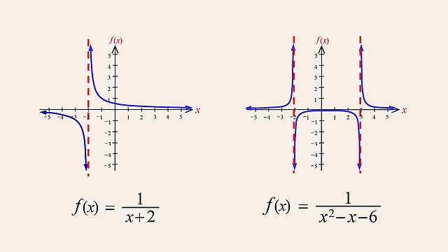
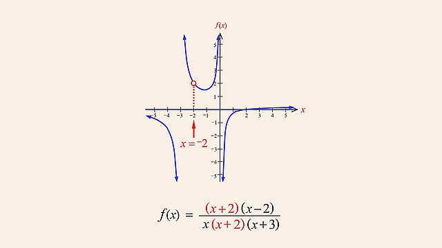
In the previous lecture, we saw examples of x values that cause a rational function's numerator to be zero, where those x values produce x-axis intercepts in the function's graph. We also saw x values that cause denominator zeros that correspond to vertical asymptotes. Since when a rational function's denominator is zero, the function's value is undefined, those x values must be excluded from the function's domain and therefore correspond to missing points in the function's graph. Although, as we saw, those missing points may be associated with vertical asymptotes, in this lecture we will see how when a numerator and denominator zero are both the same, that x value will not correspond to a vertical asymptote, but will simply cause a missing point or "hole" in the function's graph.

93. Rational Functions and Nonvertical Asymptotes
Although a rational function may have any number of vertical asymptotes or no vertical asymptotes, rational functions will always have exactly one non-vertical asymptote. Since a function's value is undefined at a vertical asymptote, its graph can approach arbitrarily close to but can never intersect a vertical asymptote. However, unlike vertical asymptotes, a function's graph may intersect or cross its non-vertical asymptote, although as x values continue to grow, the distance between a rational function's graph and its non-vertical asymptote will continue to decrease. Non-vertical asymptotes can be horizontal lines described by constant functions, slanted lines called "oblique" asymptotes described by linear functions, or curves called "curvilinear" asymptotes described by higher-order polynomial functions. In this lecture we will discuss various types of non-vertical asymptotes and show how to determine a rational function's horizontal asymptote.

94. Rational Functions with Oblique or Curvilinear Asymptotes
In the previous lecture we saw that although a rational function may have any number of vertical asymptotes or no vertical asymptotes, rational functions will always have exactly one non-vertical asymptote. Unlike vertical asymptotes, a function's graph may intersect or cross its non-vertical asymptote, although as x values continue to grow, the distance between a rational function's graph and its non-vertical asymptote will continue to decrease. Non-vertical asymptotes can be horizontal lines described by constant functions, slanted lines called "oblique" asymptotes described by linear functions, or curves called "curvilinear" asymptotes described by higher-order polynomial functions. In this lecture we will show how to determine a polynomial function that describes a rational function's oblique or curvilinear asymptote.